How to Perform Exploratory Factor Analysis (EFA) using SPSS

Exploratory Faction Analysis

Learn How to perform Exploratory Factor Analysis using SPSS. The tutorial covers in detail

  • Concept of Exploratory Factor Analysis
  • Differences between EFA and CFA
  • Key Terms in Exploratory Factor Analysis
  • Process of Conducting Exploratory Factor Analysis
  • Reporting Exploratory Factor Analysis
To see complete SPSS playlist for more tutorials, Click Here

What is Factor Analysis?

  1. Factor analysis is used as a data reduction technique.
  2. Factor analysis takes a large number of variables and reduces or summarizes it to represent them in different smaller factors, those factors are made up of the initial set of variables.
  3. Factor analysis is a method for investigating whether a number of variables of interest are related to a smaller number of unobservable factors. This is done by grouping variables based on inter-correlations among a set of variables.
  4. Those initial variables are the manifest variables/observed variables while the factors that are extracted in the process are the latent variables.
  5. A common usage of factor analysis is in developing scale/questionnaires for measuring constructs that are not directly observable in real life.
  6. The factor Analysis technique primarily examines the systematic interdependence among a set of observed variables (through correlation), and those variables, that have higher correlation are grouped together.
  7. Factor analysis helps the scholars answer the question that “How well do the items go well together? In case we are building a new Scale”.

EFA vs CFA

  • When applied to a research problem, these methods can be used to either confirm a priori established theories or identify data patterns and relationships.
  • Specifically, they are confirmatory when testing the hypotheses of existing theories and concepts and exploratory when they search for latent patterns in the data in case there is no or only little prior knowledge on how the variables are related.
  • When exploratory factor analysis is applied to a data set, the method searches for relationships (variables with high correlation are grouped together) between the variables in an effort to reduce a large number of variables to a smaller set of composite factors (i.e., combinations of variables).
  • The final set of composite factors is a result of exploring relationships in the data and reporting the relationships that are found (if any).
  • In simple words, EFA is an exploratory technique that is utilized in research to group a large number of variables (observed variables) into smaller representative factors (latent factors) whereas CFA is utilized to test a particular set of relationships based on some theory and to ascertain the data fits the proposed model in an adequate manner.

Basic Terminologies in Factor Analysis

The following is the list of some basic terms frequently used in the factor analysis

  • Kaiser-Meyer-Olkin (KMO) measure of sampling adequacy: The Kaiser-Meyer-Olkin (KMO) measure of sampling adequacy is a statistics used to examine the appropriateness of factor analysis based on the sample of the study. A high value of statistic (from 0.5 – 1) indicates the appropriateness of the factor analysis for the data in hand, whereas a low value of statistic (below 0.5) indicates the inappropriateness of the factor analysis. This means that the sample is not enough for EFA.
  • Bartlett’s test of Sphericity: Bartlett’s test of sphericity is a test statistic used to examine the hypothesis that the variables are uncorrelated in the population. In other words, the population correlation matrix is an identity matrix; each variable correlates perfectly with itself (r = 1) but has no correlation with the other variables (r = 0).
  • A value less than 0.05 indicate that the data in hand do not produce an identity matrix as with an identify matrix, factor analysis is meaningless. This means that there exists a significant relationship among the variables. A significant result (Sig. < 0.05) indicates matrix is not an identity matrix; i.e., the variables do relate to one another enough to run a meaningful EFA.
  • Communality: Communality is the amount of variance a variable shares with all the other variables being considered. Small values indicate variables that do not fit well with the factor solution, and should possibly be dropped from the analysis. Normally values Less than .50 are removed.
  • Percentage of Variance: It gives the percentage of variance that can be attributed to each specific factor relative to the total variance in all the factors.
  • Eigen Value: The eigenvalue represents the total variance explained by each factor. Factors having eigenvalues over one (1) are selected for further study.
  • Scree Plot: It is a plot of eigenvalues and factor number according to the order of extraction. This plot is used to determine the optimal number of factors to be retained in the final solution.
  • Factor Loading: Also referred to as factor-variable correlation. Factor loadings are simple correlations between the variables and the factors. Factor loadings show how well the items represents the underlying factor.
  • Factor Matrix: A factor matrix contains the factor loadings of all the variables on all the factors extracted.

Rotation Method

Makes the Loading Patterns Easy to Understand

Varimax (most common)

Minimizes number of variables with extreme loadings (high or low) on a   factor. Minimizes the correlation between factors. Makes it possible to   identify a variable with a factor. Components are always orthogonal—each   component explains non-redundant information

Direct oblimin (DO)

Factors are allowed to be correlated

Rotations that allow for correlation are called oblique rotations; rotations that assume the factors are not correlated are called orthogonal rotations.

Varimax returns factors that are orthogonal; Oblimin allows the factors to not be orthogonal.


Process of Conducting the Factor Analysis

  • Step 1: Problem Formulation
  • Step 2: EFA Requirements
  • Step 3: Appropriate Factoring Technique
  • Step 4: Decision regarding No. of Factors
  • Step 5: Factor Rotation
  • Step 6: Model Fit
  • Step 7: Running Exploratory Factor Analysis
  • Step 8: Interpretation and Reporting

Step 1: Problem Formulation

  • The first step in conducting the factor analysis is to formulate the problem of the factor analysis. As discussed earlier, the main focus of the factor analysis is to reduce data.
  • For this purpose, a researcher has to select a list of variables that will be converted into a new set of factors based on the common essence present in each of the variables.
  • For selecting variables, a researcher can take the help of literature, past research, or use the experience of other researchers or executives. for more on scale development process, please click here
  • It is important to note that the variables should be measurable on an interval scale or a ratio scale.
  • Another important aspect of the factor analysis is to determine the sample size, which will be used for the factor analysis. As a thumb rule, the sample size should be four or five times of the variable included in the factor analysis.

Step 2: EFA Requirements

  • Analyze the correlation among the variables. If there is no correlation among the variables or if the degree of correlation among the variables is very low, then the appropriateness of the factor analysis will be under serious doubt. In the factor analysis, a researcher expects that some of the variables are highly correlated with each other to form a factor.
  • Kaiser has presented the range as follows: statistic >0.9 is marvellous, >0.8 meritorious, >0.7 middling, >0.6 mediocre, >0.5 miserable, and <0.5 unacceptable.
  • Bartlett’s test of sphericity tests the hypothesis whether the population correlation matrix is an identity matrix. The existence of the identity matrix puts the correctness of the factor analysis under suspicion. P values less than .05 shows that population correlation matrix is not an identity matrix.
  • The communalities describe the amount of variance a variable shares with all other variables taken into study. Relatively small value of the communality suggests that the concerned variable is a misfit for the factor solution and should be dropped out from the factor analysis.

Step 3: Factoring Technique

  • The principal component method is the most commonly used method of data analysis in the factor analysis model.
  • When the objective of the factor analysis is to summarize the information in a larger set of variables into fewer factors, the principal component analysis is used.
  • The main focus of the principal component method is to transform a set of interrelated variables into a set of uncorrelated linear combinations of these variables.
  • This method is applied when the primary focus of the factor analysis is to determine the minimum number of factors that attributes maximum variance in the data. The obtained factors are often referred as the principal components.

Step 4: No. of Factors

  • Eigen Value: An eigenvalue is the amount of variance in the variable taken for the study that is associated with a factor. According to eigenvalue criteria, the factors having more than one eigenvalue are included in the model.
  • Scree Plot: Scree plot is a plot of the eigenvalues and component (factor) number according to the order of extraction.
  • The shape of the plot is used to determine the optimum number of factors to be retained in the final solution. The objective of the Scree plot is to visually isolate an elbow, which can be defined as the point where the eigenvalues form a liner descending trend.
  • Percentage of Variance Criteria: It gives the percentage of variance that can be attributed to each specific factor relative to the total variance in all the factors. This approach is based on the concept of cumulative percentage of variance.
  • The number of factors should be included in the model for which cumulative percentage of variance reaches a satisfactory level. The general recommendation is that the factors explaining 60%–70% of the variance should be retained in the model.

Step 5: Factor Rotation

  • After selection of factors, the immediate step is to rotate the factors. The rotated simple structure solutions are often easy to interpret, whereas the originally unextracted (unrotated) factors are often difficult to interpret.
  • A rotation is required because the original factor model may be mathematically correct but may be difficult in terms of interpretation. If various factors have a high loading on the same variable, then interpretation will be extremely difficult.
  • Rotation solves this kind of interpretation difficulty. The main objective of rotation is to produce a relatively simple structure in which there may be a high factor loading on one factor and a low factor loading on all other factors.
  • The widely applied method of rotation is the ‘Varimax procedure.’ Although a number of rotation methods have been developed, varimax has been generally regarded as the best orthogonal rotation and is overwhelmingly the most widely used orthogonal rotation in psychological research.

Step 6: Model Fit

  • The last step in the factor analysis is to determine the fitness of the factor analysis model. In factor analysis, the factors are generated on the basis of observed correlation between the variables.
  • The degree of correlation between the variables can be reproduced. For an appropriate factor analysis solution, the difference between the reproduced and observed correlation should be small (less than 0.05).
  • As a rule of thumb, ‘a model that is a good fit will have less than 50% of the non-redundant residuals with absolute values that are greater than .05’.

Step 7: Running Exploratory Factor Analysis

The Problem:

Investigate if there is any smaller number of unobservable factors in the 19 variables that measure University Social Responsibility on which the data is available. The example is based on scale development. Initial items identified to measure University Social Responsibility were 19, the researcher would like to assess if there are any underlying dimensions. 

 Steps to run Factor Analysis

  • Choose Analyze → Dimension Reduction → Factor
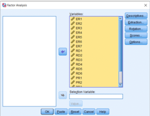
  • The resulting dialog box is shown in Figure
Menu Location Exploratory Factor Analysis in SPSS
  • Select the variables from the left-hand side box and transfer them to the box labeled Variables.

Items Dialog Box

  • Click on the Descriptives button which brings up a dialog box as shown in the figure. In the Statistics section, make sure that Initial Solution is ticked. In the section marked Correlation Matrix, select the options Coefficients and KMO and Bartlett’s test of sphericity. Click on Continue.
Factor Analysis Descriptives Section
  • Click on the button labeled Extraction which brings up a dialog box as shown in Figure.
Factor Analysis Extraction Methods
  • There are many extraction methods listed, which can be obtained by clicking on the drop-down arrow in the box against Method. Two commonly used extraction methods are Principal Components and Principal Axis Factoring. I have selected Principal Axis Factoring in this case. Also, check the Scree plot check box.
  • Next select whether we want to analyze the correlation matrix or the covariance matrix for FA. The recommended option for beginners is to use the correlation matrix, advanced users may, however, choose the covariance matrix for special cases.
  • Click against Unrotated factor solution and Scree plot to display the two in the output.
  • SPSS allows specifying the number of factors we want to extract. Default setting is to choose factors with eigenvalues greater than 1 as factors with eigenvalues less than 1 do not carry enough information. We can also specify the number of factors if we have a specific requirement to extract a certain number of factors.
Factor Analysis Extraction Options
  •  Click on Continue to return to the main dialog box.
  • Next, click on the button labeled Rotation, to specify the specific rotation strategy you want to adopt. This brings up a dialog box as shown in Figure
  • The SPSS program gives five options for rotations. Select Varimax from this box. Click on Continue to return to the main dialog box.
Factor Rotation
  • Finally click on the button labeled Options, which will bring up a dialog box as shown in Figure. It is advisable to suppress values below 0.40 as this is a standard criterion used by researchers to identify important factor loadings. We have not done this in order to present the full output.

Factor Analysis Set Minimum Loading Option

  • Click on Continue to return to the main dialog box and click on OK to run the analysis.

Step 7: Interpretation and Reporting

An EFA was performed using a principal component analysis and varimax rotation. The minimum factor loading criteria was set to 0.50. The communality of the scale, which indicates the amount of variance in each dimension, was also assessed to ensure acceptable levels of explanation. The results show that all communalities were over 0.50.

An important step involved weighing the overall significance of the correlation matrix through Bartlett’s Test of Sphericity, which provides a measure of the statistical probability that the correlation matrix has significant correlations among some of its components. The results were significant, x2(n = 215) = 2013.292 (p < 0.001), which indicates its suitability for factor analysis. The Kaiser–Meyer–Olkin measure of sampling adequacy (MSA), which indicates the appropriateness of the data for factor analysis, was 0.931. In this regard, data with MSA values above 0.800 are considered appropriate for factor analysis. Finally, the factor solution derived from this analysis yielded four factors for the scale, which accounted for 57.753 per cent of the variation in the data.

Nonetheless, in this initial EFA, two items (i.e. “RDR1: The university is involved in funding ‘relevant’ research.”, “PR1: The university is performing in a manner consistent with the philanthropic and charitable expectations of society.”) failed to load on any dimension significantly. “RDR2: Students are educated regarding their social responsibility in their area of specialization.” loaded onto a factor other than its underlying factor.  Hence, the three items were removed from further analysis.

The authors repeated the EFA without including these items. The results of this new analysis confirmed the five-dimensional structure theoretically defined in the research (see Table). The Kaiser–Meyer–Olkin MSA was 0.917. The three dimensions explained a total of 60.798 per cent of the variance among the items in the study. The Bartlett’s Test of sphericity proved to be significant and all communalities were over the required value of 0.500. The four factors identified as part of this EFA aligned with the theoretical proposition in this research. Factor 1 includes items ER1 to ER7, referring to Ethical Responsibilities (ER). Factor 2 gathers items RDR2 to RDR6, which represents Research and Development Responsibilities (RDR). Finally, Factor 3 includes items PR2 to PR6, referring to Philanthropic Responsibilities (PR). Factor Loadings are presented in table.

Reporting Exploratory Factor Analysis

For more on Exploratory Factor Analysis, Read

  • Gaur, A. S., & Gaur, S. S. (2006). Statistical methods for practice and research: A guide to data analysis using SPSS. Sage.
  • Pallant, J. (2013). SPSS survival manual. McGraw-hill education (UK).

Videos: A Step by Step Guide to Exploratory Factor Analysis

Additional SPSS Tutorials