
How to Assess Convergent Validity?
Learn the concept and process of establishing convergent validity using SmartPLS4
Understanding Convergent Validity.
This session discusses in detail the concept and assessment of Convergent Validity using SmartPLS 4. The statistic is assessed as part of the measurement model.
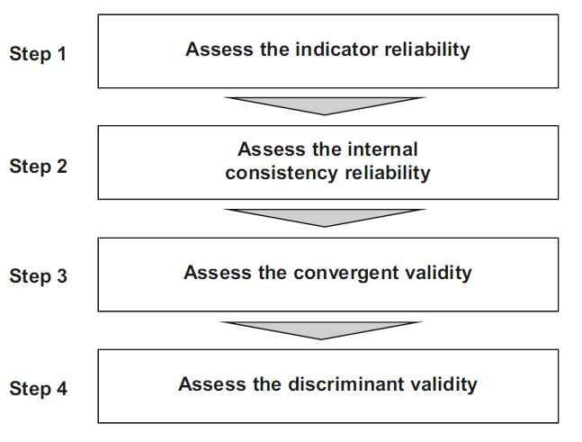
Most often, the constructs are reflective at lower level. Hence, all the lower order constructs in the study are assessed for reliability and validity. The following figure highlights the steps in measurement model assessment.In the last session we discussed how to assess Step 1 and Step 2. In this tutorial, the focus is on convergent validity (Step 3).
What is Convergent Validity?
In the preceding session, the focus was on comprehending the construct validity, delineating its concept and within this construct validity, a pivotal aspect emerged that is convergent validity. To ascertain convergent validity through Smart PLS4, a specific statistical measure comes into play, namely, the Average Variance Extracted (AVE). This discourse delves into the methodology of establishing convergent validity using Smart PLS4, along with guidance on addressing potential issues that may arise during the process.
Upon constructing a model in Smart PLS4, the initial step involves calculating the AVE values. These values serve as a yardstick, and a key consideration is whether the AVE values surpass the 0.50 threshold for each relevant construct. The AVE, derived from loadings, signifies the extent to which items converge to represent an underlying construct. Notably, a value exceeding 0.70 for each item indicates a robust representation. Accessing the AVE values can be accomplished in the report section under quality criteria.
AVE Value less than 0.50!
If, however, the AVE falls below the recommended 0.50 mark, attention must be directed towards rectifying the issue. To diagnose and address such situations, a meticulous approach is required. The graphical output provides insights into individual item loadings. Items with loadings below 0.70 are scrutinized, and if the overall AVE remains subpar, those specific items become subject to potential removal.
The calculation of AVE involves squaring the loadings for a given construct, summing these squared values, and then dividing by the number of items. An AVE value below 0.50 necessitates further evaluation. However, the decision to delete an item isn’t solely contingent on its individual loading. Items with loadings between 0.40 and 0.70 may be considered for removal only if their deletion contributes substantially to improving AVE beyond the required threshold.
A practical example (see video at the end of this page) elucidates this methodology: if an item’s loading is less than 0.40, its removal is considered. If the AVE and Composite Reliability (CR) values remain satisfactory post-removal, further deletions may not be necessary. On the contrary, persisting issues warrant a gradual approach—starting with items below 0.50, progressing to 0.60, and eventually addressing items with loadings less than 0.70. Items falling within the 0.40 to 0.70 range are potential candidates for removal, provided their elimination substantially enhances both composite reliability and AVE.
Reference
Hair Jr, J. F., Hult, G. T. M., Ringle, C. M., Sarstedt, M., Danks, N. P., & Ray, S. (2021). Partial least squares structural equation modeling (PLS-SEM) using R: A workbook.
To Download the Book, Click Here
This book is licensed under the terms of the Creative Commons Attribution 4.0 International
License (http://creativecommons.org/licenses/by/4.0/)
License (http://creativecommons.org/licenses/by/4.0/)
Video: How to Establish Convergent Validity?
Additional SmartPLS 4 Tutorials
- A Basic and Simple Model in SmartPLS4
- Basic SEM Concepts – Convergent and Discriminant Validity
- Basic Structural Equation Modelling (SEM) Concepts
- Categorical Moderation Analysis using SEMinR
- How to Assess Construct Reliability?
- How to Assess Discriminant Validity (Construct validity)
- How to Assess Reflective-Reflective Higher Order Construct
- How to Design a Measurement Model?
- How to Enter Data in SPSS or Excel
- How to Solve Discriminant Validity Issues
- How to Use Necessary Condition Analysis in SmartPLS4?
- Reflective-Formative Higher-Order Model using SmartPLS4
- Simple Structural Model in SmartPLS4
- SmartPLS4 Tutorials Series Introduction
- Steps in Data Analysis
- What is a Formative Construct?